Financial Data Analysis with Spyder

By the end of this workshop participants will be able to use Spyder effectively for applying some normative financial theories and models to assemble a portfolio of assets in a way that maximizes the expected return for a given level of risk. In this way, statistically-based tools are used to construct investment portfolios.

Prerequisites

To follow this workshop we recommend that you have a intermediate knowledge of Python. You can visit The Python Tutorial to learn the basics of this programming language or to refresh your knowledge of Python.

You will also need to have Anaconda (or Miniconda) and Spyder installed. More information about Spyder installation in installation guide.

Important

Spyder now offers Standalone installers for Windows and macOS, making it easier to get up and running with the application without having to download Anaconda or manually install it in your existing environment. While we still support Anaconda, we recommend this install method on those platforms to avoid most problems with package conflicts and other issues.

It is also desirable to have the following prior knowledge:

• Intermediate level of Python

• Basic knowledge of Statistics

• Some knowledge of Financial Econometrics is desirable

Learning goals

After completing this workshop, you should be able to:

• Apply elementary statistical analysis to stock and cryptocurrency portfolios to measure their performance

• Understand the advantages of programming with an IDE, such as inspecting variables using the Variable Explorer and interacting with plots leveraging the Plots Pane.

Learner profile

This workshop is intended for people interested in finance who want to take their first steps in Financial Analysis using Python and Spyder.

Intro

In this workshop we will obtain financial data in real-time from Yahoo! Finance API and explore financial portfolios using Econometrics and computational tools.

Why use Python for financial analysis?

Real-time analysis of historical and current financial data is essential for those investing in financial instruments. Python has a number of features that make it ideal for financial tasks:

• It is easy to learn for anyone, whether they have previous programming experience or not

• It has a variety of specialized mathematical and statistical libraries (SciPy, NumPy, Pandas) that are commonly used for financial analysis

• It can be connected to APIs for loading financial data in real time

• It is the programming language with the most resources for machine learning (supervised learning, unsupervised learning, reinforcement learning), which is one of the most useful tools for Econometrics nowadays

• It has excellent libraries for plotting

• You can use resources such as Google Colab or Binder to do your analysis in the cloud.

Why should I use an IDE?

Although you can use Python without an IDE (Integrated Development Environment), you will work much better with one. Spyder is a Scientific Integrated Development Environment written in Python, and designed by and for scientists, engineers, and data analysts. Spyder’s capabilities and its integration with Python make it perfect for financial analysis.

Introduction to financial analysis with Spyder

If you’re not familiar with Spyder, we recommend you start with our Quickstart. But if you want a summary, here’s a quick overview.

Note

If you already have experience with Spyder, you can skip this section.

Editor

The Editor is the place where you write your code and save it as a file (script). It allows you to easily persist your work. This is where you write the code you want to keep from the data analysis you do in IPython Console. Here you will also be able to read, edit and run the code from this workshop.

IPython Console

The IPython Console is the Spyder’s component where you write chunks of code that you want to experiment with. In this workshop, we are going to give you pieces of code that you can copy and run in this console.

In essence, the IPython Console allows you to execute commands and interact with data using Python.

Variable Explorer

The Variable Explorer is one of Spyder’s best features. It allows you to interactively browse and manage the objects generated in the code of the currently selected IPython Console session.

The Variable Explorer is one of the most frequently used components in this workshop. This is the pane where we will observe the data and most of the results of the analysis, except for the plots.

Plots pane

The Plots pane shows all the static graphs and images created in your IPython Console session. All plots generated by the code will appear in this component. This pane also allows you to save each graphic in a local file or copy it to the clipboard to share it with other people.

Preparation work

Before starting, you must have installed some packages and libraries needed to run the code. We recommend you to install these requirements in a virtual environment. Here we explain step by step how to do it.

Set up Conda environment

If you would like to have Spyder in a dedicated environment to update it separately from your other packages and avoid any conflicts, you can.

You can set up your environment in two different ways.

Important

We recommend creating the virtual environment with Anaconda (or Miniconda) as it integrates seamlessly with Spyder. You can find installation instructions in Anaconda documentation.

With commands

Just run the following command in your Anaconda Prompt (Windows) or terminal (other platforms), to create a new environment called financial-analysis:

$ conda create -n financial-analysis

To install Spyder’s optional dependencies as well for full functionality, use the following command:

$ conda activate financial-analysis
$ conda install -c conda-forge numpy scipy pandas matplotlib sympy cython spyder-kernels requests multitasking lxml tqdm
$ pip install -i https://pypi.anaconda.org/ranaroussi/simple yfinance
$ pip install Historic-Crypto

Important

Spyder now offers Standalone installers for Windows and macOS, making it easier to get up and running with the application without having to download Anaconda or manually install it in your existing environment.

Download the datasets

Although during the workshop we will explain how to use some APIs to download up-to-date data, you can also download the datasets in csv format from this link.

To follow this workshop you do not need to create a new directory. However, if you have downloaded the data and want to use it instead of the APIs, you must set the directory that has the downloaded data as the working directory. In order to do this, check that the working directory is correct. You should see in the upper right corner the path to the directory where you have the downloaded data. Something like this:

Setting up the virtual environment in Spyder

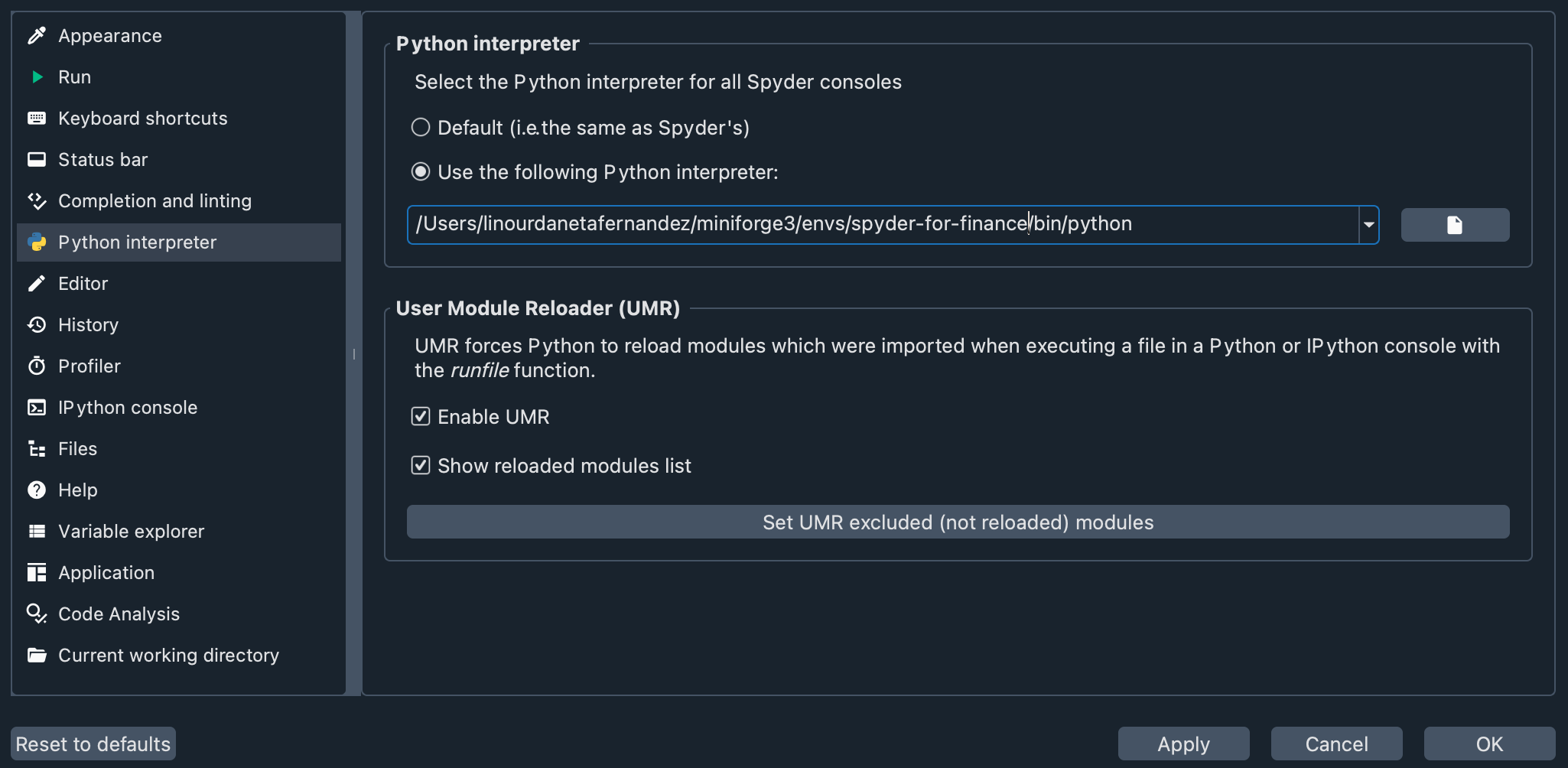
Let’s check that the virtual environment we created is enabled in Spyder. Go to Preferences > Python interpreter, and use the dropdown below Use the following Python interpreter to choose your virtual environment. You should see something like this:

Now, you have everything ready to proceed with the workshop.

Download the code

Although the workshop is designed for you to write the code in the IPython Console, we have created a file that you can download here. This script provides all the code you will write in this workshop, and you can use it as a guide if you get lost.

Obtain financial data

When it comes to finance, being up to date is very important. So we are going to use a Python library that allows us to get updated historical Stock Market records from Yahoo! Finance API. In this way, we will be able to download data in the period of time we are interested in analyzing.

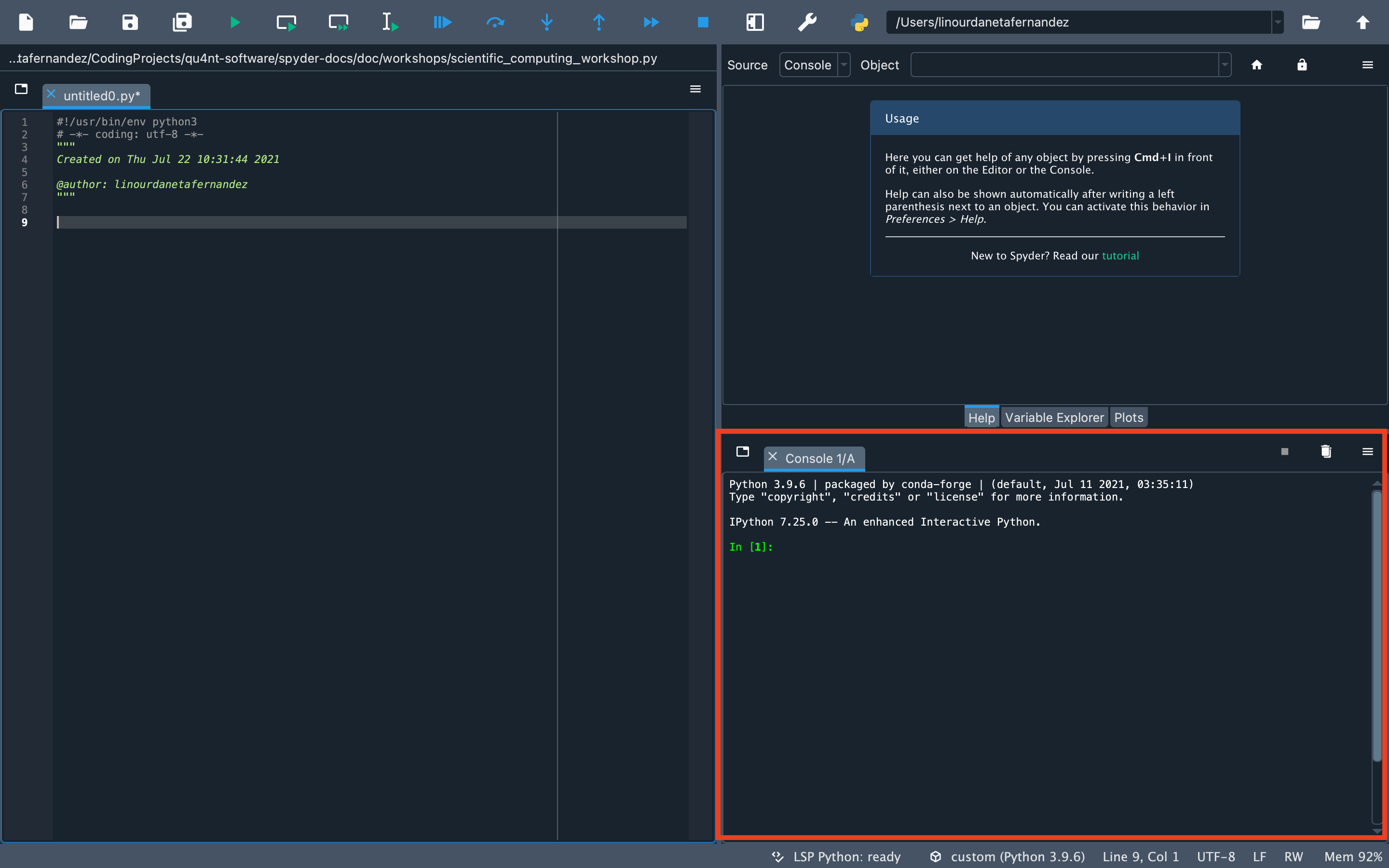
Remember to type and run all code for this workshop in the “IPython Console” at the bottom right of Spyder.

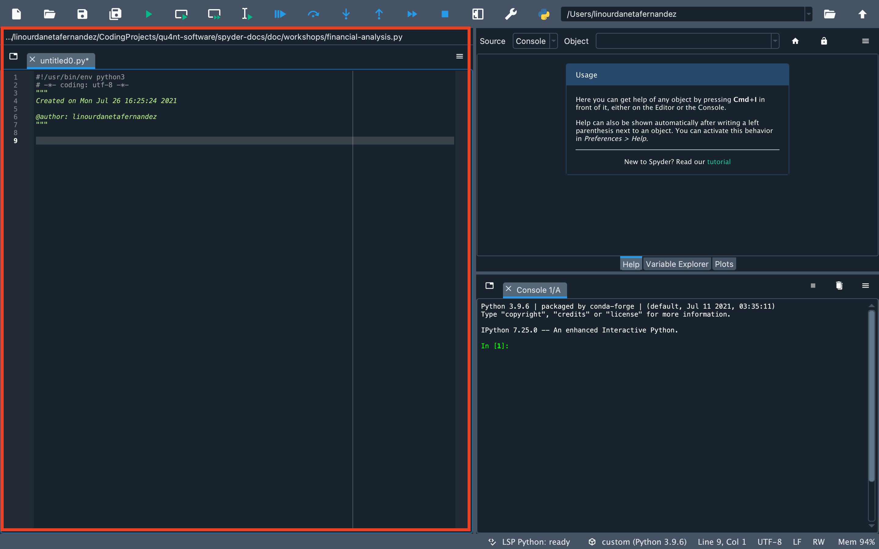
You can also write your code in the Editor (the pane that occupies the entire left side of Spyder). If you use the Editor, you can run the code by selecting it and pressing the Run selection or current line button in the Run toolbar or by pressing the F9 key.

To get started, import the libraries.

import numpy as np
import pandas as pd
import matplotlib as mpl
from scipy.optimize import minimize
import matplotlib.pyplot as plt
import pprint

from Historic_Crypto import Cryptocurrencies
from Historic_Crypto import HistoricalData
import yfinance as yf

The first group of imports is for basic operations. The second (Historic_Crypto and yfinance) imports the libraries that we will use to download financial data.

Let’s start exploring libraries with an example. We are going to get financial information about Netflix with one line of code:

netflix = yf.Ticker("NFLX")

We have used the Ticker class of the yfinance library to create a netflix object. This object contains attributes and methods that we can query to obtain various types of information.

General stock information

If you want to know which methods and attributes you can query, you can do so with the built-in help() function.

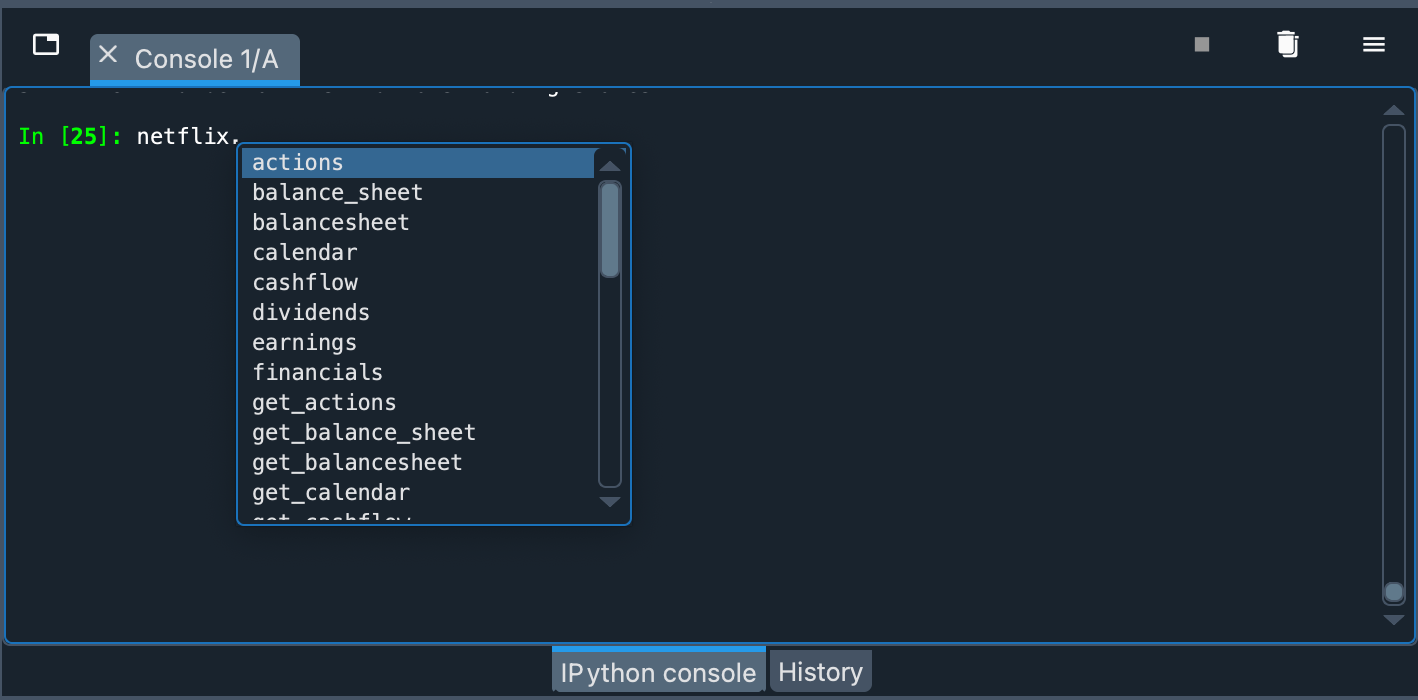
You can also type the name of the object (netflix) in the console, then type a period and hit the Tab key once. IPython suggestions will then appear to help you navigate the object:

For example, we can obtain general information with the info property of the object.

netflix_info = netflix.info

We can observe the result in the Variable Explorer, in the netflix_info variable.

If we double-click on it, a new window with detailed information will be displayed.

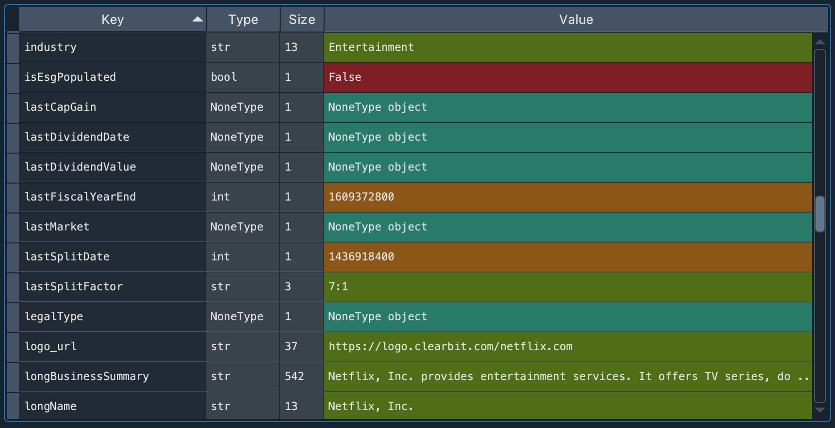
In that window we can see a Python dictionary in which each key has a value assigned to it. Each type of value is represented by a distinctive color. For example, we see that Netflix is an Entertainment industry, the summary of the business type, among other indicators. The Variable Explorer is a very convenient way to view these types of results. We can compare it to viewing them in the IPython Console with the pprint function:

pprint.pprint(netflix_info)

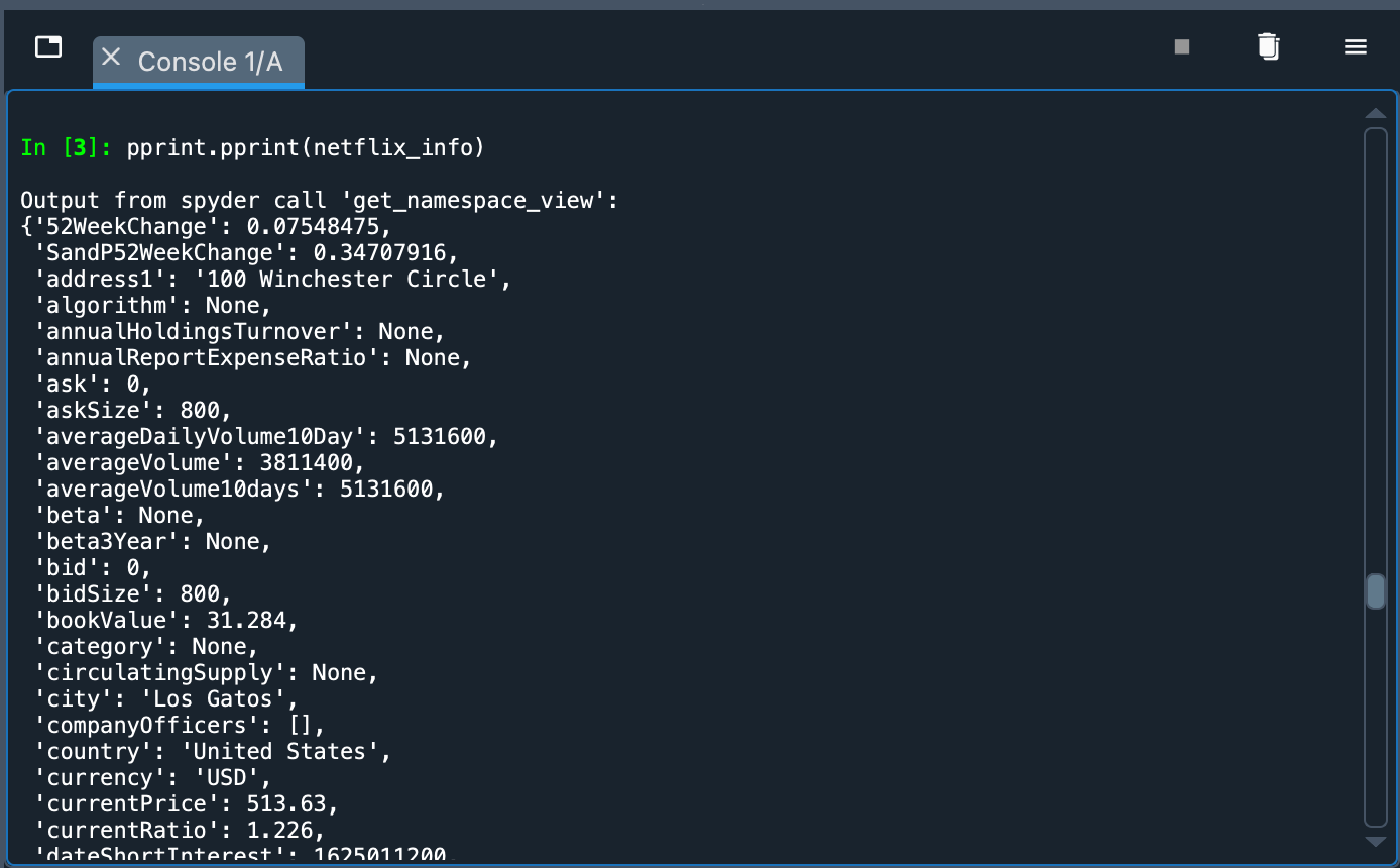
Although pprint displays all the information, it is easier to view it in the Variable Explorer.

Historical stock data

We can download in a dataset the history of a stock with the following line of code:

hist = netflix.history(period="max")

We can see a summary and more details of this dataset in the Variable Explorer. It appears as a DataFrame object, with 7 columns and thousands of rows. If we double-click on it we will see the historical records of Netflix stock organized by ascending dates.

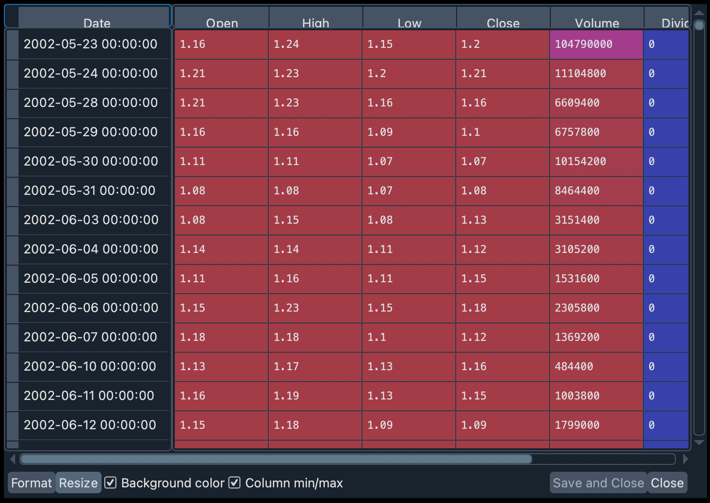
Throughout this workshop we will use this historical information to compare, with various normative financial theories, different types of financial portfolios.

First portfolio

Let’s build our first stock investment portfolio! Say we are interested in investing in technology, and we want to know what performance can be obtained by putting money into some of the “heavyweights” in this industry.

To measure the performance of our first portfolio we are going to use a classic theory in the world of finance: mean-variance portfolio (MVP) theory. This model assumes that investors only care about expected returns and the variance of such returns. The analysis is based entirely on statistical measures based on a time series of share prices, such as periodic mean returns and the variances of those returns with the same periodicity.

Prepare portfolio data

Before we start, let’s run some lines of code to style the plots. These lines are optional, but we recommend that you run them so that the graphics look like the screenshots we present in this workshop.

plt.style.use("fivethirtyeight")
mpl.rcParams["savefig.dpi"] = 300
mpl.rcParams["font.family"] = "serif"
np.set_printoptions(precision=5, suppress=True, formatter={"float": lambda x: f"{x:6.3f}"})

Suppose we want to measure the performance of a portfolio consisting of Google, Apple, Microsoft, Netflix and Amazon stocks. Let’s call this set SYMBOLS_1.

SYMBOLS_1 = ["GOOG", "AAPL", "MSFT", "NFLX", "AMZN"]

Note

If you search for SYMBOLS_1 in Variable Explorer you will not find it: Python interprets this element not as a variable, but as a constant. This is because the name is written with uppercase letters (no letter is lowercase). By default, the Variable Explorer doesn’t show this, but actually you can change the settings in the Preferences to be able to see these constants.

We are going to download the historical data for this portfolio. To do this, we are going to use the yfinance download() function, which takes as its first argument a string with the symbols (SYMBOLS_1) defined above. The rest of the arguments are the start date (start="2012-01-01"), the end date (end="2021-01-01") and how the data will be grouped (group_by="Ticker").

data_1 = yf.download(" ".join(SYMBOLS_1), start="2012-01-01", end="2021-01-01", group_by="Ticker")

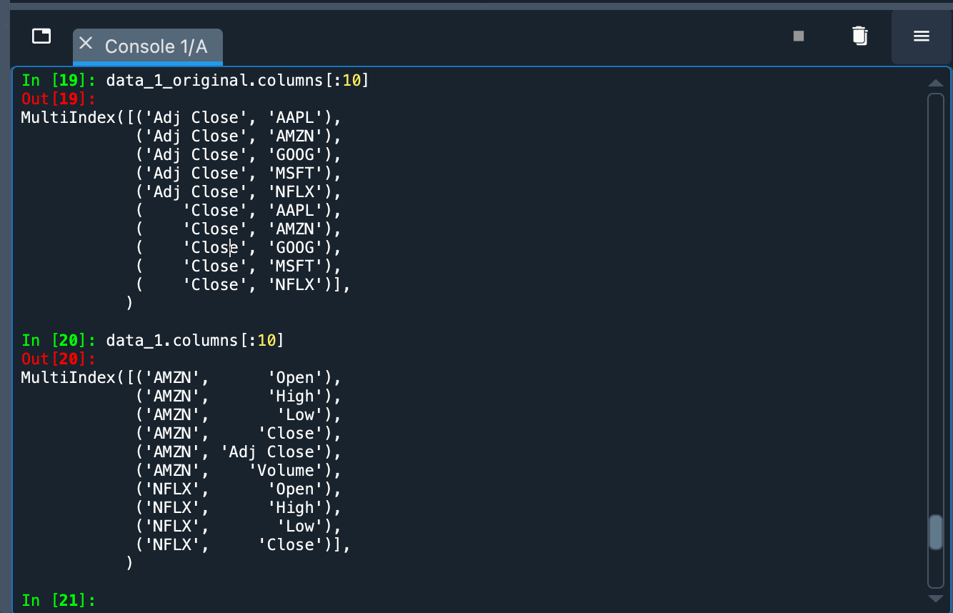
The last argument (group_by="Ticker") groups the information mainly by stock. Otherwise, the primary grouping is done by the type of information (e.g., opening price, closing price, volume traded) of the transactions. In the following image you can see the differences (above is the default organization and below is the grouping by “Ticker”).

The historical data has been downloaded as a Pandas DataFrame. We can explore this data in the variable data_1 in the Variable Explorer.

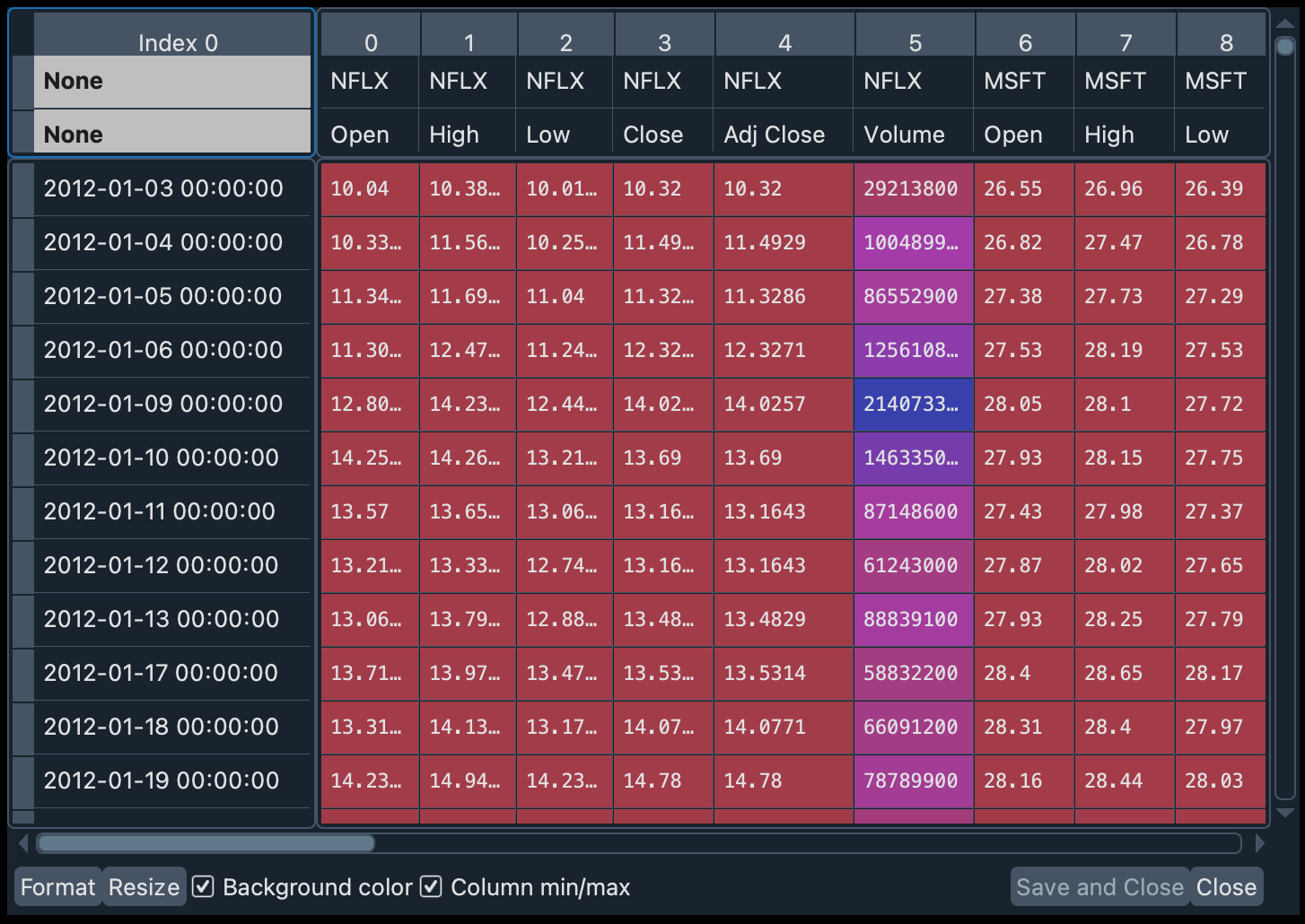
Let’s change the formatting of the data a bit so that the symbols appear as the column names, and the Ticker moves from columns to rows. We will do this with the stack() operation of the DataFrame.

data_1 = data_1.stack(level=1).rename_axis(["Date", "Ticker"]).reset_index(level=1)

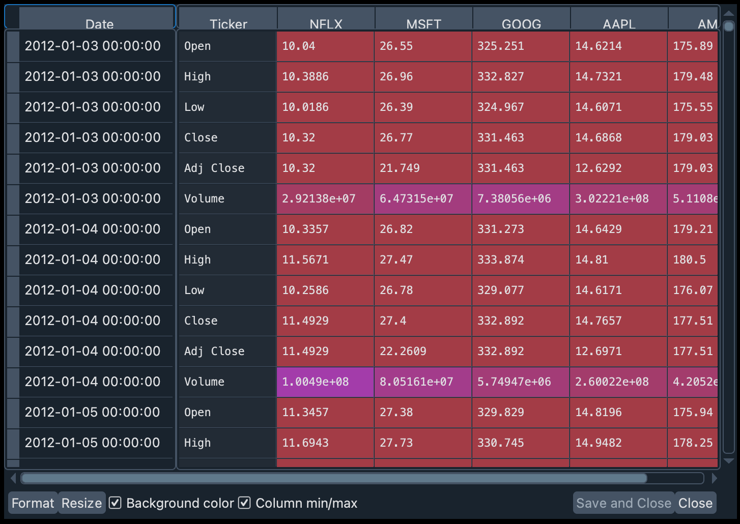
From the Ticker we are only interested in the daily closing price. So we will leave only the values for "Close" and eliminate the Ticker column afterwards.

close_data_1 = data_1[data_1.Ticker == "Close"].drop("Ticker", inplace=False, axis=1)

You will notice that there is a new DataFrame in the Variable Explorer called close_data_1 with 2,265 rows and 5 columns.

A first glance at the portfolio

We want to see how our portfolio would have performed if we had invested in it from 2012 to early 2021. How could we obtain this measurement? Let’s look at the monthly closing prices of each stock. To do this we will do an automatic resample of the data. And then we will calculate the change in relative frequencies (percentages).

The resampling will be performed with the resample("M") method and the calculation of percentages with the pct_change() method. The result will be stored in the monthly_data_1 variable.

monthly_data_1 = close_data_1.resample("M").ffill().pct_change()

Since each stock is a column, we can use the mean() method on the DataFrame to see the results.

monthly_data_1.mean()

# AMZN    0.029931
# GOOG    0.018784
# MSFT    0.020698
# AAPL    0.023033
# NFLX    0.042060
# dtype: float64

Important

Remember that this closing information represents the relative growth of each stock, not its closing price in any currency.

As we can see, all the results are positive, so this portfolio has been profitable over the years. In relative terms, the biggest gains would come from Netflix (0.4 percent). These percentages show an average of the monthly variation of the stock price. But how stable have that prices been? To find this out, we can calculate the standard deviation of stock price growth:

monthly_data_1.std()

# AMZN    0.082308
# GOOG    0.061057
# MSFT    0.058395
# AAPL    0.081239
# NFLX    0.145416
# dtype: float64

The highest volatility is found in Netflix (0.1454), which indicates that its price, despite being the fastest growing, has also had a lot of variation during these years. The most stable price, on the other hand, has been Microsoft’s (0.0583).

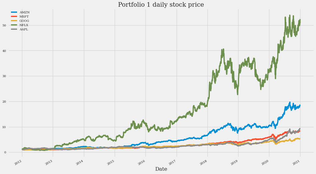
A good way to observe both growth and variability is to draw a time-series plot. To scale the values, we are going to divide the relative frequency of the closing price of the actions by the initial value it has in the dataframe close_data_1 (these initial values can be found with close_data_1.iloc[0])). The plot is drawn with the plot() method of the Pandas DataFrame (to which we pass as arguments the size of the plot and the plot title).

(close_data_1/close_data_1.iloc[0]).plot(figsize=(16, 10), title="Portfolio 1 daily stock price")

Important

You will be able to see the graph in the Plots pane. On the left, you will see the plot in detail. On the right, a stack will be created with all the plots that are generated both in the Console and by running the code directly in the Editor. You can copy, delete or save the plot to disk by clicking on it with the right mouse button or trackpad.

The above time-series plot clearly shows the growth of all stocks, particularly Netflix. The high volatility discussed above can also be seen. For example, it can be seen from the plots that, due to high volatility, investing in Netflix in the years 2014 and 2019 left virtually no profit (if shares were bought at the beginning of the year and sold right at the end).

We can also plot with the plot() method the DataFrame we already have with the monthly data. To do this, we will add 1 to all the values and calculate the accumulated product with the cumprod() method:

(monthly_data_1 + 1).cumprod().plot(figsize=(16, 10), title="Portfolio 1 monthly stock price")

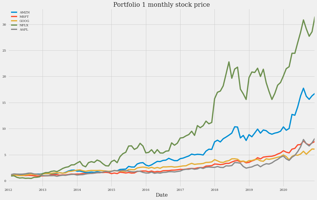
This plot of the monthly data is “smoother” than the plot of the daily data.

Returns and volatility

Remember that in the mean-variance portfolio theory what matters are the expected returns and variances. To calculate these returns, we will divide the price of the stock on one day by the price of the same stock on the previous day. We will do this by dividing the close_data_1 DataFrame by a version of itself in which we shift each record one date backwards (shift(1)). For example, if on the date 2012-01-03 a stock was valued at 1, and on the next day (2012-01-02), it was valued at 2, then in our shifted dataset, on the day 2012-01-03 the stock would be worth 1. In this way, we would divide 1 by 2. And so on with all the values of all the shares. We will also normalize the results by passing them to a logarithmic scale with np.log().

Note

Trend lines are more easily drawn in logarithmic scale because they tend to fit better to the minimums. In addition, the logarithmic scale gives a more realistic view of price movements.

rets_1 = np.log(close_data_1/close_data_1.shift(1)).dropna()

In the variable rets_1 you can see the resulting DataFrame. If you double-click on the variable name in the Variable Explorer, you will see that there are positive values (the share price increased) and negative values (the price decreased at the time of closing).

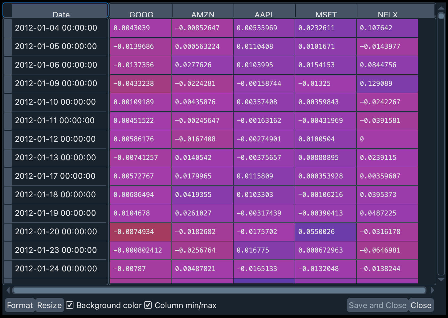
In addition to the returns of each stock, we will need the specific weight of each stock in the portfolio, i.e., how many shares of each company are in the portfolio. In this workshop we will assume that there is one share of each company and, therefore, the weights will be distributed equally.

Note

A stock is a financial security that represents that you own a part of a company (whatever the size of this part). A share, on the other hand, is the smallest unit of denomination of a stock. A stock is composed of one or several shares.

This weight will be a vector (Python list) composed of the relative weight (between 0 and 1) of each stock in the portfolio. The sum of these weights has to be 1. Since we will assume that each stock is a single share, the distribution will be equal: [0.2, 0.2, 0.2, 0.2, 0.2].

weights_1 = [0.2, 0.2, 0.2, 0.2, 0.2]

With this information we can calculate the expected return of this portfolio. The math is simple: this is given by the dot product of the portfolio weights vector and the vector of expected returns. This result must be multiplied by the number of days for which the return is to be calculated (a year has approximately 252 stock price closings).

Let’s put all this into a function:

def portfolio_return(returns, weights):
    return np.dot(returns.mean(), weights) * 252

Let’s look at the expected return of this portfolio if we hold it for one year:

portfolio_return(rets_1, weights_1)

# 0.2859066023606343

An expected gain of almost 30% in one year. Not bad, right? But don’t forget the other side of this coin: volatility. This calculation is a bit more complex. First, the dot product of the annualized covariance of the returns (this is multiplied by the number of trading days in a year) and the weights is calculated. Then the dot product of the weights and the previous result is obtained. Finally, the square root of this result is extracted. Let’s implement this into a function as well.

def portfolio_volatility(returns, weights):
    return np.dot(weights, np.dot(returns.cov() * 252, weights)) ** 0.5

Let’s see how our portfolio performs with respect to its volatility:

portfolio_volatility(rets_1, weights_1)

# 0.23704031354688784

If high return is desirable, high volatility is undesirable. The risk of this portfolio is relatively large.

Sharpe ratio

The Sharpe ratio or index is a measure of portfolio performance. It relates the portfolio’s return to its volatility, comparing the expected/realized return with the expected/realized risk. It is calculated as the difference between the actual investment returns and the expected return in a zero-risk situation, divided by the volatility of the investment. It provides a model of the additional amount of returns received for each additional unit of risk.

Let’s formalize this in a function:

def portfolio_sharpe(returns, weights):
    return portfolio_return(returns, weights) / portfolio_volatility(returns, weights)

And let’s apply this to our portfolio.

portfolio_sharpe(rets_1, weights_1)

# 1.2061518063427656

Important

The Sharpe ratio measure is best understood in context: when comparing two or more portfolios, the one with the higher Sharpe ratio provides more profit for the same amount of risk.

We can also use a Monte Carlo simulation to randomize the weights of each stock in the portfolio so that we can see the range over which the Sharpe ratio can vary. In this way we can plot some scenarios that together will give us a good insight of the relationship between expected returns and expected volatility.

We are going to do this with a function that we will explain step by step in the monte_carlo_sharpe function explained section.

def monte_carlo_sharpe(returns, symbols, weights):

    sim_weights = np.random.random((1000, len(symbols)))
    sim_weights = (sim_weights.T / sim_weights.sum(axis=1)).T

    volat_ret = [(portfolio_volatility(returns[symbols], weights), portfolio_return(returns[symbols], weights)) for weights in sim_weights]
    volat_ret = np.array(volat_ret)

    sharpe_ratio = volat_ret[:, 1] / volat_ret[:, 0]

    return volat_ret, sharpe_ratio

Warning

You do not need to type the following code in the IPython Console. If you write the function above it will be enough. It is just a code presentation to explain what is inside the function.

monte_carlo_sharpe function explained

Let’s now break the function down to understand what is happening. First, we create a numpy array of length 1,000 and width of the number of shares in the portfolio. Each row of the array has random weights that always add up to 1:

sim_weights = np.random.random((1000, len(symbols)))
sim_weights = (sim_weights.T / sim_weights.sum(axis=1)).T

The next section calculates the volatility and returns for the new random weights using a list comprehension. The resulting list is transformed back into a numpy array:

volat_ret = [(portfolio_volatility(returns[symbols], weights), portfolio_return(returns[symbols], weights)) for weights in sim_weights]
volat_ret = np.array(volat_ret)

Finally, we obtain the Sharpe ratio by dividing the index 1 (volatilities) by the index 0 (returns) of the numpy array:

sharpe_ratio = volat_ret[:, 1] / volat_ret[:, 0]

Using the monte_carlo_sharpe function

We use the function to get the simulated returns and volatility of portfolio 1 (port_1_vr) and the related Sharpe ratios (port_1_sr).

Enter the following code in the console.

port_1_vr, port_1_sr = monte_carlo_sharpe(rets_1, SYMBOLS_1, weights_1)

Note

Remember that the weights are initialized randomly, so each time you run this code you will get different results.

With this we obtain two arrays with 1,000 simulated cases for our portfolio. But the best way to explore this is with a plot.

plt.figure(figsize=(16, 10))
fig = plt.scatter(port_1_vr[:, 0], port_1_vr[:, 1], c=port_1_sr, cmap="cool")
CB = plt.colorbar(fig)
CB.set_label("Sharpe ratio")
plt.xlabel("expected volatility")
plt.ylabel("expected return")
plt.title(" | ".join(SYMBOLS_1))

You should see in the Plots pane something like this:

A roughly linear relationship can be observed between returns and volatility: the higher the volatility, the higher the gains. And the Sharpe ratio shows an important amount of variability (it is noticeable in the “width” of the line drawn).

This seems to be a good portfolio because it has a good performance with a not very large variance.

Optimal portfolio weights

Can we use the data obtained to calculate the optimal weights for the portfolio by year? Of course we can. Let’s start by delimiting the previous years as variables.

start_year, end_year = (2012, 2020)

We will now write a function to calculate these optimal weights.

def optimal_weights(returns, symbols, actual_weights, start_y, end_y):

    bounds = len(symbols) * [(0, 1), ]
    constraints = {"type": "eq", "fun": lambda weights: weights.sum() - 1}
    opt_weights = {}

    for year in range(start_y, end_y):
        _rets = returns[symbols].loc[f"{year}-01-01":f"{year}-12-31"]
        _opt_w = minimize(lambda weights: -portfolio_sharpe(_rets, weights), actual_weights, bounds=bounds, constraints=constraints)["x"]
        opt_weights[year] = _opt_w
    return opt_weights

Let’s describe this function in broad strokes. bounds indicates the maximum and minimum weights for each stock in the portfolio. The lowest weight will be 0 and the highest weight will be 1 for each stock in the portfolio. constraints is a function that ensures that the sum of the weights of all actions always adds up to 1. Then a loop is initialized that will segment the data for each year. In the variable _rets the returns for the specified year are obtained. In _opt_w the portfolio_shape() function is used to calculate the weights that maximize the Sharpe ratio. This is done with the minimize() function of SciPy (which takes as arguments the portfolio_shape function, the actual weights of our stocks in the portfolio, and the bounds and the constraints variables). Notice the - sign before portfolio_sharpe? It’s because minimize() aims to find the minimum value of a function relative to a parameter, but we are interested in the maximum, so we make the result of portfolio_sharpe a negative one.

We will use the function we just defined to calculate the optimal weights for each year, and we are going to save the result in a Pandas DataFrame to take advantage of the Variable Explorer display options.

opt_weights_1 = optimal_weights(rets_1, SYMBOLS_1, weights_1, start_year, end_year)
port_1_ow = pd.DataFrame.from_dict(opt_weights_1, orient='index')
port_1_ow.columns = SYMBOLS_1

Double click on the port_1_ow variable in the Variable Explorer. In the table, you can specify the number of decimal places to display, by clicking the format button at the bottom left of the pane, as you can see in the following image:

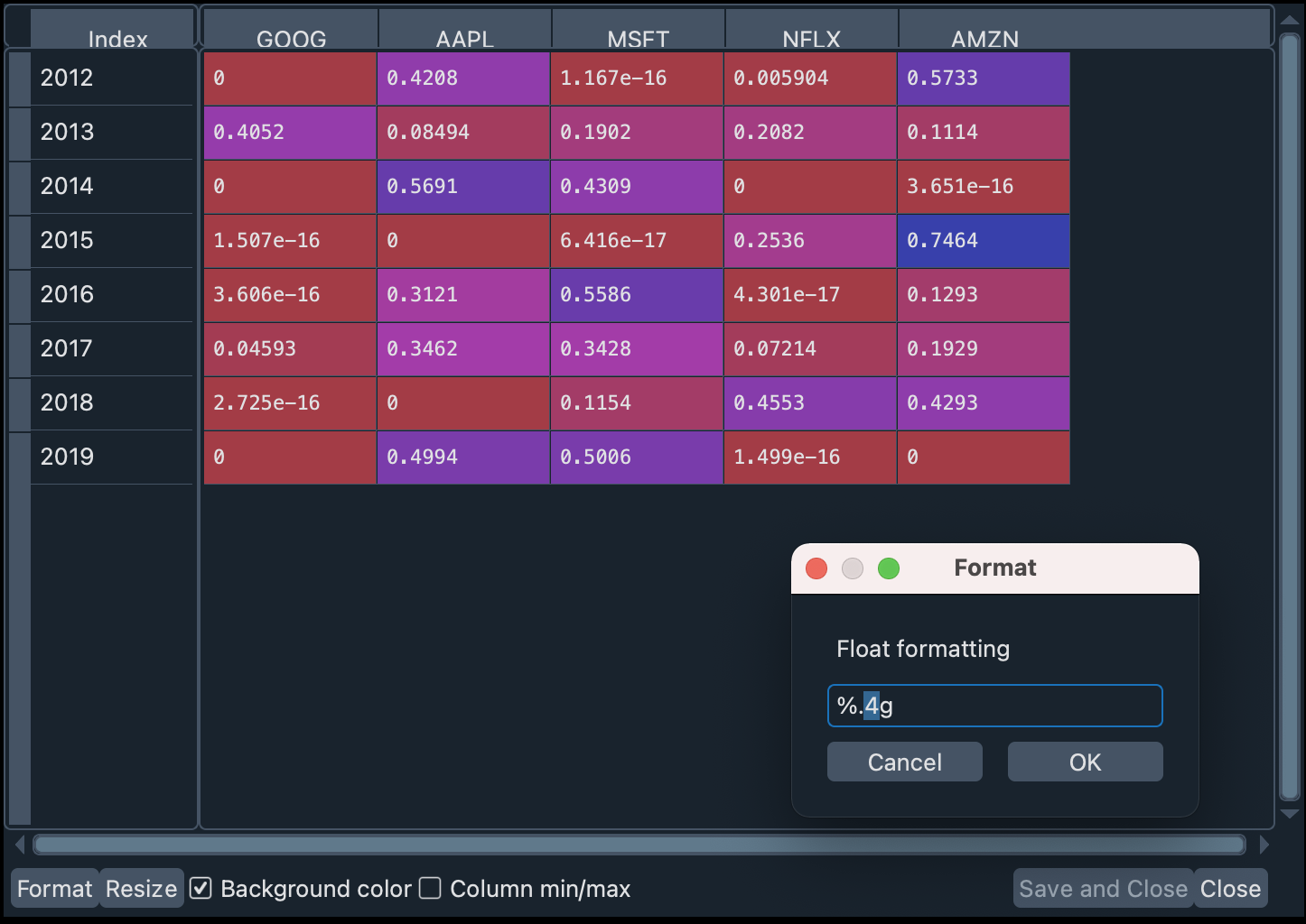
We set the number of decimal places to 4 and uncheck the Column min/max checkbox to better appreciate the contrasts in the row values (years).

You can see, for example, how 2015 was a particularly good year for investing in Amazon and Netflix, while 2014 was the year of Apple. Despite Netflix’s rapid growth over the years, its high volatility means that its Sharpe Ratio is not very remarkable in any year, especially (as we said above) in 2014 and 2019. In the same respect, Apple and Microsoft seem to be safer bets in the return/volatility ratio.

Comparison of expected and realized returns

Finally, we will use the optimal weights to calculate the expected returns and compare them with the actual returns.

def exp_real_rets(returns, opt_weights, symbols, start_year, end_year):

    _rets = {}
    for year in range(start_year, end_year):
        prev_year = returns[symbols].loc[f"{year}-01-01":f"{year}-12-31"]
        current_year = returns[symbols].loc[f"{year + 1}-01-01":f"{year + 1}-12-31"]
        expected_pr = portfolio_return(prev_year, opt_weights[year])
        realized_pr = portfolio_return(current_year, opt_weights[year])
        _rets[year + 1] = [expected_pr, realized_pr]

    return _rets

In this function we compare year to year realized returns with theoretically expected returns. This is done by estimating:

1. The returns from applying the optimal weights of the previous year’s stocks to the data for that same year (expected_pr).

2. The returns from applying the optimal weights of the previous year’s stocks to the following year’s data (realized_pr).

We are going to apply this function to the data in portfolio 1 and store the results in a DataFrame that we can review in the Variable Explorer.

port_1_exp_real = pd.DataFrame.from_dict(exp_real_rets(rets_1, opt_weights_1, SYMBOLS_1, start_year, end_year), orient='index')
port_1_exp_real.columns = ["expected", "realized"]

The expected column shows the predicted values if the optimal portfolio composition had been used. The realized column, on the other hand, shows the actual profits that would have been obtained with those weights. It can be seen that there are notable differences in some years. Let’s look at this in a plot.

port_1_exp_real.plot(kind="bar", figsize=(16, 10),title="Expected vs. realized Portfolio Returns")

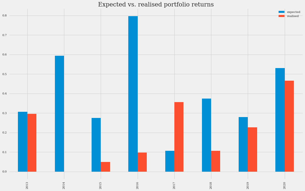
The most notable differences are seen in 2014 and 2016. In those years, the previous year’s optimal portfolio weights (in blue in the above plot) are a lousy indicator of the following year’s stock performance (in red). In 2013, our model estimated that Google and Netflix were excellent investments. But by 2014 their share price did not grow if we compare the price at the beginning and at the end of that year. And something similar happened in 2016, in which Amazon’s growing trend of the previous year diminished, and the value of Microsoft and Apple shares grew.

Let’s summarize these numbers.

port_1_exp_real.mean()

# expected    0.408009
# realized    0.199700
# dtype: float64

Our optimal weight model offered us a profit of around 40%, but the profit we would have obtained, due to real market fluctuations, would have been almost 20%. Not bad, but the mean-variance portfolio model we have applied for annual calculations is not very accurate, is it?

And this result is less encouraging if we calculate the correlations between expected and realized profits.

port_1_exp_real[["expected", "realized"]].corr()

#           expected  realized
# expected  1.000000 -0.324053
# realized -0.324053  1.000000

As we can see, the correlations are negative, which warns us that we should be cautious when using this type of modeling.

Second portfolio

We are now going to apply all the previous code with a portfolio of a different nature. Let’s assume that instead of technology companies, we are now interested in pharmaceuticals. We will build a portfolio with stocks of Pfizer, Astra Zeneca, Johnson & Johnson.

Download the data

Let’s download the data and format it.

SYMBOLS_2 = ["PFE", "AZN", "JNJ"]  # Pfizer, Astra Zeneca, Johnson N Johnson

data_2 = yf.download(" ".join(SYMBOLS_2), start="2012-01-01", end="2021-01-01", group_by="Ticker")
data_2 = data_2.stack(level=1).rename_axis(["Date", "Ticker"]).reset_index(level=1)

close_data_2 = data_2[data_2.Ticker == "Close"].drop("Ticker", inplace=False, axis=1)

Note

If you do not want to use the yfinance API, you can download the close_data_2.csv file containing the closing information for this portfolio. Copy this file to your working directory. Load the data with the following instruction: >>> close_data_2 = pd.read_csv("close_data_2.csv").

Mean and standard deviation

We are going to put the data in a monthly format and observe the mean and standard deviation.

monthly_data_2 = close_data_2.resample("M").ffill().pct_change()

print("Mean:")
print(monthly_data_2.mean())
print("STD:")
print(monthly_data_2.std())

# Mean:
# AZN    0.008778
# PFE    0.006954
# JNJ    0.009126
# dtype: float64
# STD:
# AZN    0.063068
# PFE    0.053174
# JNJ    0.044063
# dtype: float64

As in portfolio 1, all means are positive. But its largest value (that of JNJ) barely reaches 1% per month, which is slower growth than that of portfolio 1. The variation is also smaller compared to that of the previous portfolio (here the largest deviation is 0.06) which makes it a lower risk investment.

Daily and monthly timelines

Let’s better visualize the above with a couple of charts.

rets_2 = np.log(close_data_2[SYMBOLS_2] / close_data_2[SYMBOLS_2].shift(1)).dropna()

(close_data_2[SYMBOLS_2] / close_data_2[SYMBOLS_2].iloc[0]).plot(figsize=(16, 10), title="Portfolio 2 daily stock price")

fig = plt.figure()
(monthly_data_2 + 1).cumprod().plot(figsize=(16, 10), title="Portfolio 2 monthly stock price")

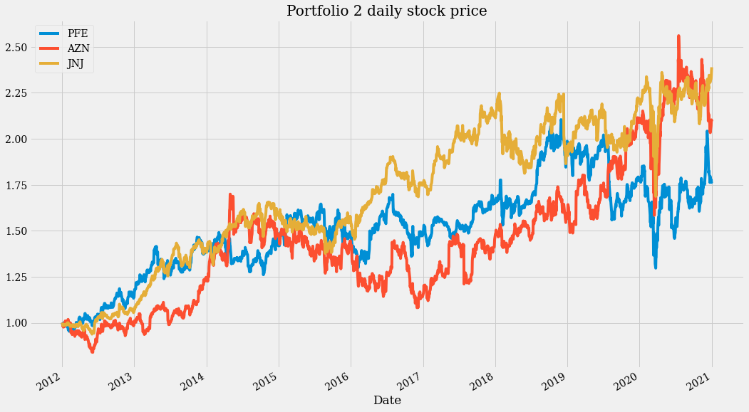
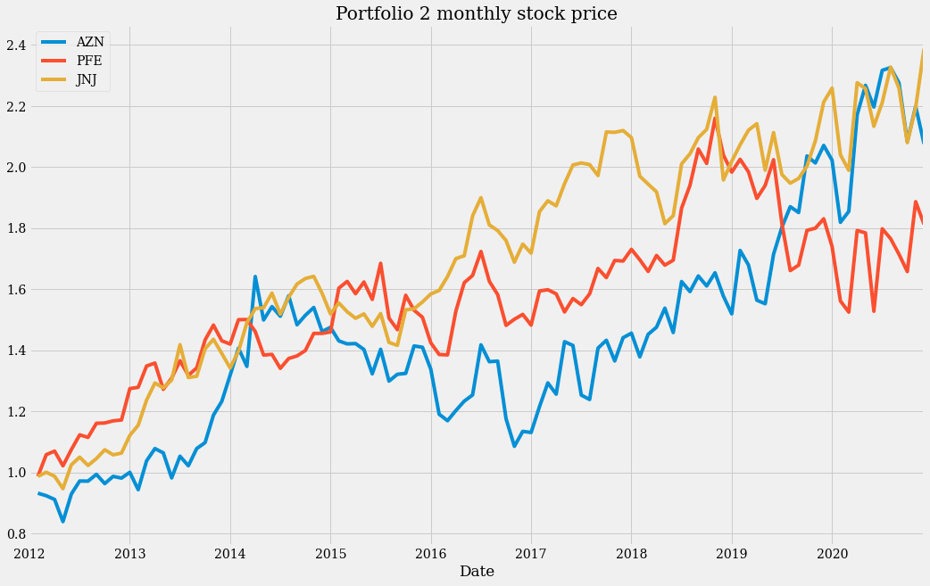
These two plots show a steady growth over the years, but also a high variability in each year. This seems to be a good portfolio only if taken as a long-term investment.

Returns, volatility and Sharpe ratio

To confirm what was said in the previous section, let’s calculate returns, volatility and Sharpe ratio.

weights_2 = len(close_data_2.columns) * [1 / len(close_data_2.columns)]

print(f"Portfolio 2 returns: {portfolio_return(rets_2, weights_2):.4f}")
print(f"Portfolio 2 volatility: {portfolio_volatility(rets_2, weights_2):.4f}")
print(f"portfolio 2 Sharpe: {portfolio_sharpe(rets_2, weights_2):.4f}")

# Portfolio 2 returns: 0.0809
# Portfolio 2 volatility: 0.1637
# Portfolio 2 Sharpe: 0.4940

The return of this portfolio is significantly lower than that of the previous portfolio (0.0809 < 0.2859). Its volatility (0.1637 < 0.2370) is also lower, but to a lesser extent. This is reflected in a lower Sharpe ratio as well (0.4940 < 1.2062). This means, within the mean-variance theory approach, that the first portfolio is a better investment than the second one.

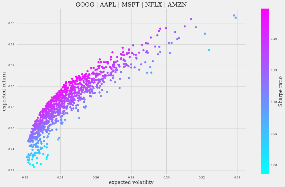
The different behavior is clearly observed if we apply a Monte Carlo simulation and visualize it with a graph:

port_2_vr, port_2_sr = monte_carlo_sharpe(rets_2, SYMBOLS_2, weights_2)

plt.figure(figsize=(16, 10))
fig = plt.scatter(port_2_vr[:, 0], port_2_vr[:, 1], c=port_2_sr, cmap="cool")
CB = plt.colorbar(fig)
CB.set_label("Sharpe ratio")
plt.xlabel("expected volatility")
plt.ylabel("expected return")
plt.title(" | ".join(SYMBOLS_2))

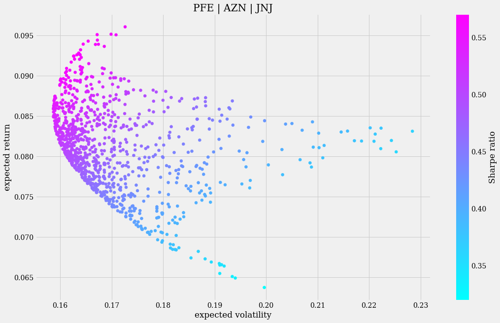
High volatility does not correspond in most cases with high returns. In fact, there are scenarios in the simulation in which higher expected returns are related to lower expected volatility.

Optimal pharmaceutical stock weights

Let us now see what are the optimal weights for each stock using the optimal_weights function.

start_year, end_year = (2012, 2020)
opt_weights_2 = optimal_weights(rets_2, SYMBOLS_2, weights_2, start_year, end_year)

port_2_ow = pd.DataFrame.from_dict(opt_weights_2, orient='index')
port_2_ow.columns = SYMBOLS_2

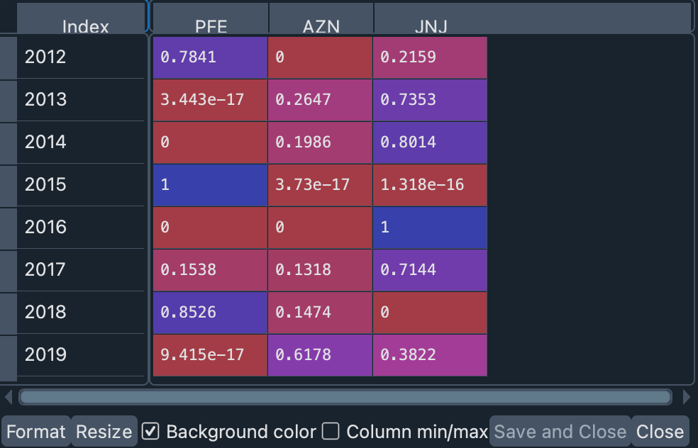
In addition, we can use these optimal weights to plot the expected and realized returns of this portfolio for each year.

port_2_exp_real = pd.DataFrame.from_dict(exp_real_rets(rets_2, opt_weights_2, SYMBOLS_2, start_year, end_year), orient='index')
port_2_exp_real.columns = ["expected", "realized"]

port_2_exp_real.plot(kind="bar", figsize=(16, 10),title="Expected vs. realized portfolio returns")

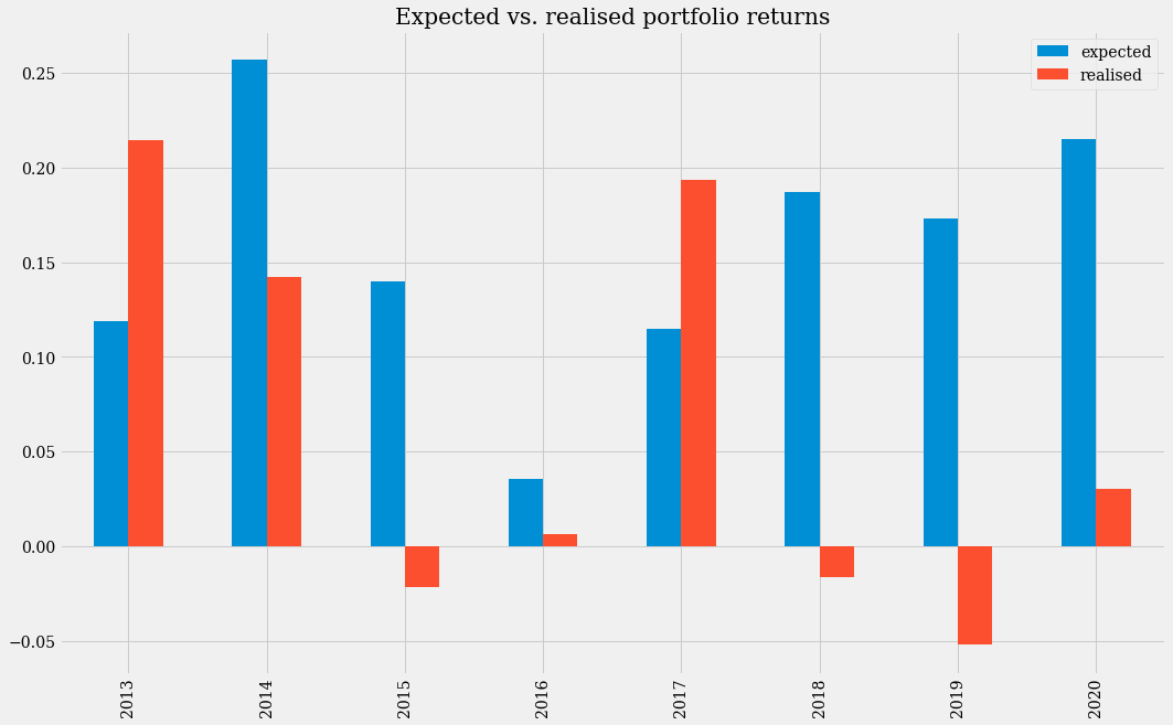
Due to the high volatility of this portfolio, our model has not been able to adequately forecast expected returns in several of the years. Higher than expected returns would have been realized in 2013 and 2017, but in 2015 and 2018 using the model would have generated losses.

Finally, let us look at the differences between the expected and realized means, and the linear correlation between the data.

print("Expected and realized means:")
print(port_2_exp_real.mean())
print("Expected and realized correlations:")
print(port_2_exp_real[["expected", "realized"]].corr())

# Expected and realized means:
# expected    0.155103
# realized    0.062207

# Expected and realized correlations:
#          expected  realized
# expected  1.000000 -0.023134
# realized -0.023134  1.000000

As we can see, the model with optimal weights predicted a return close to 15% per year, but the realized return would have barely reached 6%. And the negative correlations show, as with portfolio 1, that there does not seem to be any correspondence between these values.

The comparison is then favorable for portfolio 1. But what if we compare portfolio 1 with a “higher risk” investment such as cryptocurrencies? Let’s discuss it below.

Third portfolio

Download cryptocurrencies data

Our third portfolio will consist of three cryptocurrencies: bitcoin (BTC), ethereum (ETH) and litecoin (LTC). To access historical data, we are going to use a library called Historic-Crypto.

Important

If you want to make use of the data without the Historic-Crypto library, you can download the dataset “crypto_hist.csv” in your working directory, and load it in memory with the instruction crypto_hist = pd.read_csv("crypto_hist.csv"), and skip to section Monthly data.

Import the libraries:

from Historic_Crypto import Cryptocurrencies
from Historic_Crypto import HistoricalData

We are going to use the Cryptocurrencies class to obtain a list of available cryptocurrencies.

crypto_list = Cryptocurrencies(coin_search="", extended_output=True).find_crypto_pairs()

Note

If you want more information about the use of this library you can make a quick query using the Spyder Help panel (type in the console Cryptocurrencies and use Ctrl-I or Cmd-I to display it). Or you can read the documentation in their official repository

A new variable has appeared in the Variable Explorer: crypto_list. It is a Pandas DataFrame that has a basic description of the types of cryptocurrency transactions. For example, we can look up which token is the token for ethereum transactions in US dollars.

crypto_list.loc[crypto_list.base_currency == "ETH"]

In this case, we are interested in the symbol with ID 171: ETH-USD.

We can use the HistoricalData class of Historic-Crypto to download the history of transactions done in the cryptocurrencies of our portfolio, in US dollars.

# Download and format ETC data:
ETC_HIST = HistoricalData("ETH-USD", 3600 * 24, "2016-01-01-00-00", "2021-01-01-00-00").retrieve_data()
ETC_HIST.rename(columns={"close": "ETC"}, inplace=True)
ETC_HIST.drop(["low", "high", "open", "volume"], axis=1, inplace=True)


# Download and format BTC data:
BTC_HIST = HistoricalData("BTC-USD", 3600 * 24, "2016-01-01-00-00", "2021-01-01-00-00").retrieve_data()
BTC_HIST.rename(columns={"close": "BTC"}, inplace=True)
BTC_HIST.drop(["low", "high", "open", "volume"], axis=1, inplace=True)


# Download and format LTC data:
LTC_HIST = HistoricalData("LTC-USD", 3600 * 24, "2016-01-01-00-00", "2021-01-01-00-00").retrieve_data()
LTC_HIST.rename(columns={"close": "LTC"}, inplace=True)
LTC_HIST.drop(["low", "high", "open", "volume"], axis=1, inplace=True)

Let’s merge the resulting dataframes to have all the data in a single table.

crypto_hist = pd.merge(BTC_HIST, ETC_HIST, on=["time"])
crypto_hist = pd.merge(crypto_hist, LTC_HIST, on=["time"])

We will not present the procedures and code in this section, but only the results of the analysis. You can follow the steps in the previous sections to recreate these results.

Note

Use all this section on portfolio 3 to check your understanding of the concepts and code we have presented until now. If you have any questions, you can consult the code code that accompanies this workshop. But we encourage you to try as much as possible to solve the code on your own.

Monthly data

Let’s take a look at the monthly history of cryptocurrency price growth.

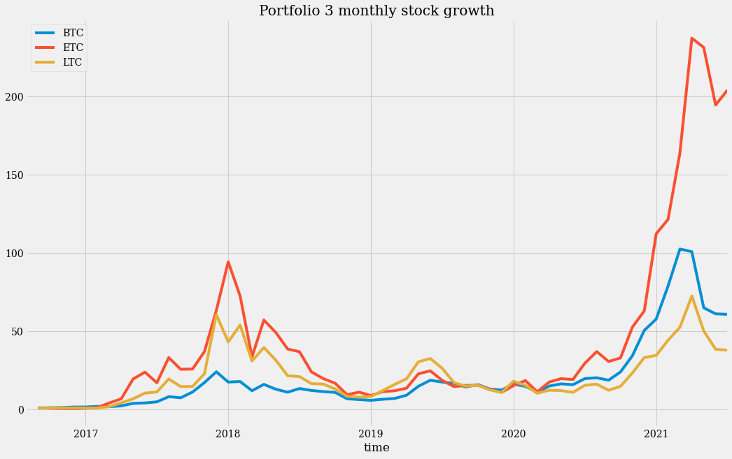
We can note that the scale here is much larger. And the proportion of ETH growth over the other two coins is quite remarkable.

Return, volatility and Sharpe ratio

Let’s consider the return, volatility and Sharpe ratio of this portfolio.

• Return: 0.6203

• Volatility: 0.7587

• Sharpe: 0.8176

These numbers are higher than those obtained for portfolios 1 and 2, except for the Sharpe ratio. This is a very volatile portfolio (in fact three times more volatile than that of the technology companies), and that makes it ultimately not as profitable as portfolio 1. The returns are higher (almost double) but the risk may not compensate for it.

Monte carlo simulation

The Monte Carlo simulation also shows the non-linear correlation between risk and returns (as you can see, sometimes high risk involves only modest profits):

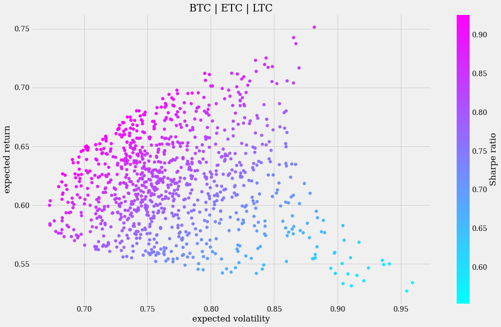
As can be seen, there are points (bottom right) that show a very high volatility and yet have a very low expected return. In this sense, portfolio 1 represents a safer investment because the higher risk is consistently offset by higher returns.

Optimal cryptocurrency weights

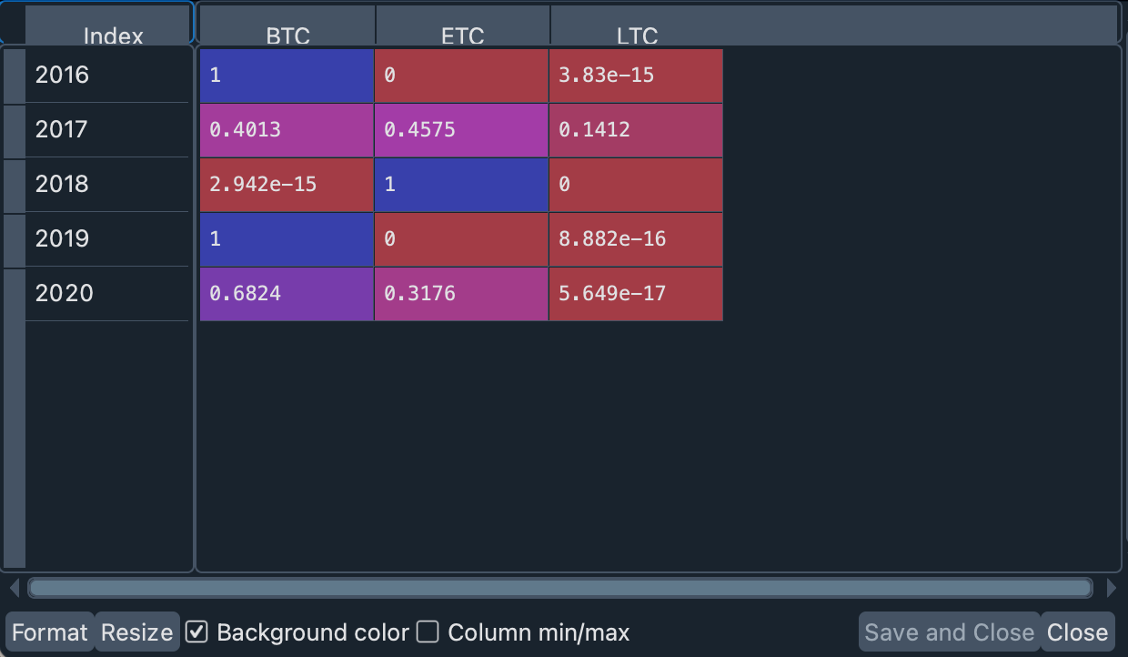
The optimal portfolio weights, if calculated annually, suggest that our portfolio should have been quite polarized in some years: the recommendation is to have bought only bitcoins before the start of 2016 and 2019, and only ethereum in 2018. Starting 2017 and 2020, on the other hand, our weights recommended a more balanced investment between bitcoin and ethereum. Litecoin is not recommended by our model.

Expected and realized returns

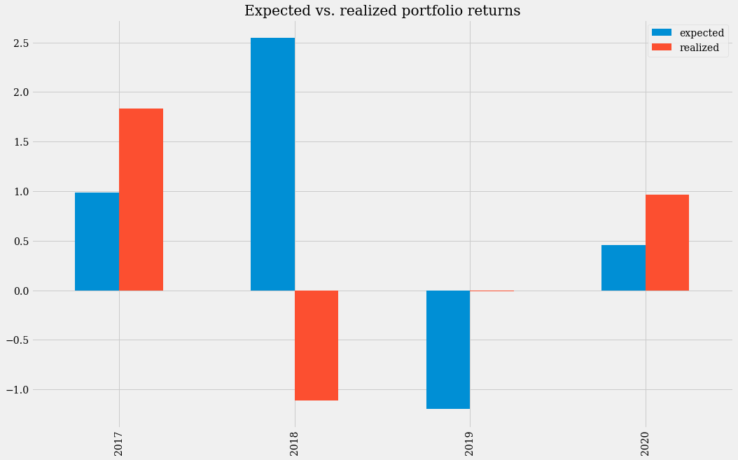
In this graph we can see that in 2017 and 2020 the earnings obtained would have exceeded the expected earnings (with our calculated weights). In 2019 our model predicted a sharp drop in the portfolio, but in reality the portfolio did not make either annualized gains or losses that year. In contrast, in 2018, our model would have brought us heavy losses, as the value of cryptocurrencies declined sharply that year.

The mean expected return for our portfolio is 0.6972, which is higher than the realized return of 0.4181 that we would have obtained. Having invested in this portfolio over the long term (from 2016 to the present) would have been a very good deal. Due to the high variability, investing in the short term would have been very risky. In terms of gross profits, the realized returns of this portfolio were more than double those of portfolio 1 (0.4181 > 0.1997).

Final words

The mean-variance portfolio (MVP) theory is one of the many tools available to financial analysis. In recent years, machine learning algorithms have even been used to predict the behavior of stock prices more accurately than can be achieved with any standard financial theory.

The examples given during this workshop are not intended to serve as guidelines for you to invest your money. It is only a first step towards learning financial analysis using Python and a scientific IDE.

In this workshop you have learned how to:

• Set up a Conda environment.

• Use the Spyder Editor to write and run code.

• Write and test code with the IPython Console.

• Obtain financial data using an API.

• Graphing data.

• Inspect objects in the Variable Explorer.

• Browse between plots using the Plots pane.

• Manipulate data in a Pandas DataFrame.

• Build a financial portfolio.

• Calculate returns and volatility of a portfolio over time.

• Obtain the optimal weights of the stocks in a portfolio.

With the skills learned here, you will be able to approach more complex topics of financial analysis such as those you will find in the references in the next section.

Thank you for reaching the end of this workshop! We hope you found it helpful and informative.

If you are interested in an introduction to scientific computing with Spyder, you can visit the workshop Scientific Computing and Visualization with Spyder.

Homework

If you want to check what you have learned, we suggest you try to obtain the results presented for the third portfolio. If you have any questions, you can consult the code that accompanies this workshop in our repository.

Further reading

Much of the math used to apply MVP was the mathematics outlined in Yves Hilpisch’s excellent book, which we recommend to you:

• Yves Hilpisch, Y. (2020). Artificial Intelligence in Finance. O’Reilly.*

A classic that has been with us for decades and is one of Warren Buffett’s favorites:

• Graham, B. (1949). The Intelligent Investor. HarperCollins.

Another good resource for financial analysis with Python is the following book by James Ma Weiming:

• Ma Weiming, J. (2019). Mastering Python for Finance. Packt